Setting up a computational chemistry research environment
Table of Contents
Over the past two years, while working on my PhD @geem-lab in UFSC, there were several moments in which new students (undergrads, M.Sc. and Ph.D students new to computational chemistry) came by and me and my colleagues had to go around and teach them how to set up a basic chemistry research environment in linux.
Inspired by this experience, and noticing that there were no comprehensive tutorials to set up this kind of envinronment (at least with the tools that me and my fellow Ph.D. colleagues have been using), I decided to write this post to teach a non-proeficient linux user how to set up all the basic software needed to start a journey in computational chemistry.
Although I’m focusing on linux, as I believe computational chemistry is a democratic, empowering and cheap way of doing science, I’ll do my best to include Windows users by adding relevant links to installation instructions on this platform.
Also, I wanna preface this by saying that we will be focusing on things at a lower scale, so we will be focusing on small molecules, and bigger things such as proteins are for now out of scope, which means that software for molecular dynamics simulations such as AMBER, GROMACS and LAMMPS wont be installed here. (They might be a theme for the future though)
What we are aiming for at the end of this article#
The idea is to give in this article a tutorial to install the three main softwares we use on our day-to-day research in our laboratory, by the end of the article you will have all the tools you need and a very quick overview on how to use each one of them.
Following articles will show how to obtain spectroscopic data using these 3 tools. :)
What we’ll need#
So, to start we need just 4 different pieces of software (we could actually start just with the vizualizer and XTB):
- A terminal emulator
- A molecular vizualizer
- A very handy semi-empirical, CLI package called XTB
- Orca, our main software suite for doing calculations
In case you’re using windows, you can follow along by installing WSL, if you opt to use this tool, the only moment we will diverge is when installing the molecular vizualizer. But do know that everything that I’m installing here can also be installed natively for windows, I just think that it is much more simpler and powerfull to use these tools in a UNIX terminal.
So, let the journey begin.
Installation#
Basic utilities in the terminal#
There are good reasons to use a terminal instead of a graphical user interface (a GUI), I shall not enter those thoughts as it’s not the best opportunity, but do know that after I started using it I never went back, it’s just so more efficient to interact with the computer in this way.
Anyways, in the terminal we will need some basic utilities, I will assume you’re rocking an ubuntu as your OS, in which case you can run the following command:
sudo apt install vim gcc make build-essential libssl-dev zlib1g-dev libbz2-dev libreadline-dev libsqlite3-dev wget curl llvm libncursesw5-dev xz-utils tk-dev libxml2-dev libxmlsec1-dev libffi-dev liblzma-dev linux-headers-$(uname -r)
Not every single one of these programs will be used here, bit trust me, it is good to have these installed in your system.
Depending on the OS you’re using this command might differ a little bit, but
I bet that you either are using something that uses apt such as ubuntu, mint, or
some kind of derivative of debian, or you know what package manager your system uses.
Installing the molecular vizualizer#
If you’re on windows this is the easy part, just go to chemcraft website and download the .exe installer. Linux users will do the same, though we have some steps before executing it, as we will install it through wine. Wine is a way to use windows programs in linux, and we will use it because chemcraft for linux is kinda broken.
So let us install wine, I will give here as an example the directions for ubuntu, if you’re on a differente operating system (or if you want to follow along the original documentation where I’m getting this from, click here) please chek the link provided and work your way from there. (It probably wont differ much from this)
sudo dpkg --add-architecture i386
sudo mkdir -pm755 /etc/apt/keyrings
sudo wget -O /etc/apt/keyrings/winehq-archive.key https://dl.winehq.org/wine-builds/winehq.key
Now we need to get our ubuntu version, so run the following command:
cat /etc/os-release
For instance, the output I receive is the following:
PRETTY_NAME=“Ubuntu 22.04.3 LTS” NAME=“Ubuntu” VERSION_ID=“22.04” VERSION=“22.04.3 LTS (Jammy Jellyfish)” VERSION_CODENAME=jammy ID=ubuntu ID_LIKE=debian HOME_URL=“ https://www.ubuntu.com/" SUPPORT_URL=“ https://help.ubuntu.com/" BUG_REPORT_URL=“ https://bugs.launchpad.net/ubuntu/" PRIVACY_POLICY_URL=“ https://www.ubuntu.com/legal/terms-and-policies/privacy-policy" UBUNTU_CODENAME=jammy
So I know my ubuntu version is 22.04. Now depending on your version you will run a different command.
- Ubuntu 23.10
sudo wget -NP /etc/apt/sources.list.d/ https://dl.winehq.org/wine-builds/ubuntu/dists/mantic/winehq-mantic.sources
- Ubuntu 23.04
sudo wget -NP /etc/apt/sources.list.d/ https://dl.winehq.org/wine-builds/ubuntu/dists/lunar/winehq-lunar.sources
- Ubuntu 22.04
sudo wget -NP /etc/apt/sources.list.d/ https://dl.winehq.org/wine-builds/ubuntu/dists/jammy/winehq-jammy.sources
- Ubuntu 20.04
sudo wget -NP /etc/apt/sources.list.d/ https://dl.winehq.org/wine-builds/ubuntu/dists/focal/winehq-focal.sources
Great, now everything is set up and we can install wine.
sudo apt update && sudo apt install --install-recommends winehq-stable
After all this, we now have wine available! Check that it’s working by running
wine --version
Now, if you have not yet downloaded the chemcraft .exe for windows, do it know. We will execute the installer using wine. If you downloaded the chemcraft installer in ~/Downloads, for instance, navigate to the directory and execute the installer, like so:
wine ./Chemcraft_b688bt_win64.exe
Follow the GUI installer, and just remember in which folder chemcraft is being installed on, probably it will be ~/.wine/drive_c/.
After installation, to confirm everything is working as expected, run the following command:
wine ~/.wine/drive_c/Chemcraft/Chemcraft.exe
After this, chemcraft should start. For a final convenience, as it is really boring to keep writing this whole .wine/drive_c…. path every time we want to launch chemcraft, you can register the following alias:
alias chemcraft='wine ~/.wine/drive_c/Chemcraft/Chemcraft.exe'
After reloading your config (source ~/.bashrc), you should be able
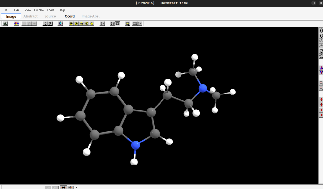
to launch chemcraft by just typing chemcraft in your terminal, you should see something like this:

To draw a molecule, one option is to go into the fragment section by typing Ctrl-f (or by clicking in Edit -> Fragments in the top menu). Draw something to test it out! I decided to draw DMT (because well, why not…) and to do this i first added an indole ring, and then used the -R- section in the fragments to add an ethyl fragment, and then added an -NH2 followed by the two methyls, obtaining our dear friend represented bellow:
Great! Now to proceed with any calculations on other software, we will need the xyz
coordintes of this little beauty. To get them you can go the coord tab on the
top, then click on coords format on the bottom and change that to XMOL format (symbol x y z),
then copy those coordinates to a text file with .xyz extension, we will use this later
on XTB and orca.
Installing XTB#
Great, now we are done installing our molecular viewer and the next step is getting software to run our simulations!
One thing you might have noticed, and is a shame on part of the chemcraft developer (we truly need a modern molecular viewer…), is that there is no way to optimize a structure inside the molecular viewer. In other words, you can draw any nonsense structure and there is no way to obtain a plausible structure for it.
In our workflow this is a place where the XTB suite is already really usefull (there are many more). So lets install it.
If you want to check for yourself the documentation and see how the developers advise to install the software, this is the best way! From now on, I will provide the manner in which I installed and which I find the best, which is through the binary given in the XTB release page.
Find the xtb-6.6.1-linux-x86_64.tar.xz file and download it somewhere. Then, navigate to
the folder where you’ve downloaded the file and issue the following command:
tar -xvf ./xtb-6.6.1-linux-x86_64.tar.xz
Now, I personally keep all software in the /opt folder, but you can leave the extracted folder
anywhere you want, you’ll just have to adapt some configuration below.
So, if you wanna keep it in /opt:
sudo mv ./xtb-6.6.1-linux-x86_64.tar.xz /opt/xtb
Do note that I changed the folder name to xtb. After this, we need to specify some stuff in our ~/.bashrc file,
(If you’re still in doubt about how this file works click here)
you can do that by both, opening your ~/.bashrc file in a text editor, or issuing the following command:
echo "export XTBHOME=/opt/xtb source\n$XTBHOME/share/xtb/config_env.bash" >> ~/.bashrc
Now if you reload your configurations (source ~/.bashrc) and type xtb and hit enter, you should
see the following:
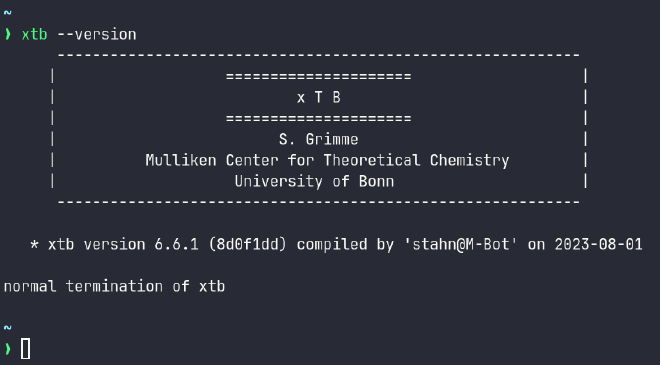
Which means XTB is now installed and ready to go! yay!
Now just for a test drive, lets see how well XTB can calculate an IR spectrum for the molecule we drew previously using chemcraft (test this with the molecule you drew!) In case you did not save the xyz coordinates, or want to test out with the DMT molecule I drew, here are the xyz coordinates, copy it to a file (like init.xyz or something like that)
30
symmetry c1
C       -0.869713548      0.000000000     -3.620281775
C       -0.869713548     -0.661620007     -2.379491185
C       -0.869713548      0.118696949     -1.188749095
C       -0.869713548      1.517490905     -1.210112686
C       -0.869713548      2.139727367     -2.452691172
C       -0.869713548      1.388227459     -3.646058299
C       -0.869713548     -2.040455663     -1.974306861
C       -0.869713548     -2.058324587     -0.605078227
N       -0.869713548     -0.761110969     -0.125045297
H       -0.869713548     -0.569660768     -4.545443682
H       -0.869713548      2.097112517     -0.291140122
H       -0.869713548      3.224412090     -2.505441965
H       -0.869713548      1.908128210     -4.599549412
H       -0.869713548     -2.894567717      0.079261227
H       -0.869713548     -0.500851598      0.847136555
C       -0.869713548     -3.275729247     -2.893925898
H        0.007856452     -3.234299727     -3.555193423
H       -1.747283548     -3.234299727     -3.555193423
C       -0.869713548     -4.607890091     -2.134880001
H        0.007856452     -4.649319612     -1.473612477
H       -1.747283548     -4.649319612     -1.473612477
N       -0.869713548     -5.787014876     -3.012698173
C       -1.420006420     -7.008103571     -2.406876291
H       -2.319937240     -7.344517616     -2.934188877
H       -0.694690801     -7.829225031     -2.434882405
H       -1.693509864     -6.844932428     -1.358220143
C       -1.420006420     -5.556867349     -4.356241947
H       -0.625372305     -5.503192762     -5.109092607
H       -2.100975071     -6.363040706     -4.652001577
H       -1.981789910     -4.616952355     -4.401714852
Once you have the xyz file (saved as something like init.xyz), you can run the following command:
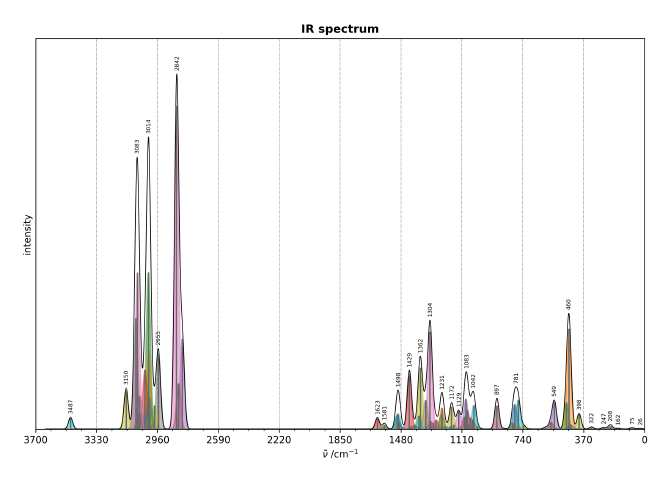
xtb init.xyz --ohess
This will optimize and generate a vibspectrum file. If you want to plot it, I have a script which the plots xtb vibspectrum file to a spectra in png like the following:
Installing orca#
Just with a molecular viewer and XTB we can already do a lot of very nice simulations! But when dealing with small molecules (while AI methods don’t take over), DFT is the king in the hill. And to be able to use DFT, we will rely on ORCA, which is free for academics. =)
To start, head over to the ORCA forum and create your account. After that, and confirming your account in your email, you will be able to access the downloads section. Choose the latest version and download the three .tar.xz files.
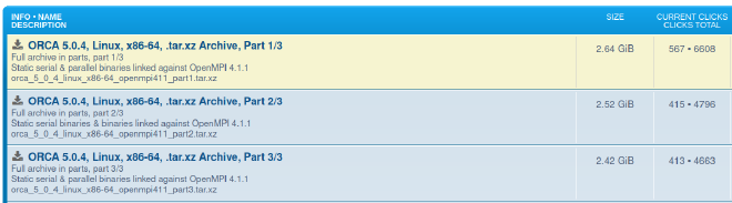
After downloading them, create a directory called orca and move the three .tar.xz files there:
mkdir orca
mv orca*.tar.xz orca/
Enter the directory, then extract the three tar.xz as we did previously:
tar -xvf *.tar.xz
After extracting the three files, we can move the folder somewhere we like just as we did with XTB, in my case I also keep orca in /opt:
cd ..
sudo mv orca /opt
Great! Now just with some configuration we will already be able to use orca as well. As we did with XTB,
we also need to specify some variables in our ~/.bashrc file, so add the following lines in it:
export PATH=/opt/orca:$PATH
export LD_LIBRARY_PATH=/opt/orca:$LD_LIBRARY_PATH
or alternatively:
echo "export PATH=/opt/orca:$PATH\nexport LD_LIBRARY_PATH=/opt/orca:$LD_LIBRARY_PATH"
After sourcing our ~/.bashrc file again, we are ready to go! To test if everything works fine,
run your orca binary from the command line with the full path to it:
/opt/orca/orca
And you should see something like this:
Great! Now to submit our first calculation, let us also obtain an ir-spectra now from orca. To do this, we first need to create in input file to orca, which also contains xyz coordinates but needs some more directives.
Below is a sample optimization input for orca which was built using an input generator that I wrote recently, we basically need to tell orca which functional we wish to use, as well as the basis set and the type of calculation we are performing. (which are the opt and freq keywords)
! BP86 def2-svp
! Opt freq D3BJ

*xyz 0 1
C       -0.869713548      0.000000000     -3.620281775
C       -0.869713548     -0.661620007     -2.379491185
C       -0.869713548      0.118696949     -1.188749095
C       -0.869713548      1.517490905     -1.210112686
C       -0.869713548      2.139727367     -2.452691172
C       -0.869713548      1.388227459     -3.646058299
C       -0.869713548     -2.040455663     -1.974306861
C       -0.869713548     -2.058324587     -0.605078227
N       -0.869713548     -0.761110969     -0.125045297
H       -0.869713548     -0.569660768     -4.545443682
H       -0.869713548      2.097112517     -0.291140122
H       -0.869713548      3.224412090     -2.505441965
H       -0.869713548      1.908128210     -4.599549412
H       -0.869713548     -2.894567717      0.079261227
H       -0.869713548     -0.500851598      0.847136555
C       -0.869713548     -3.275729247     -2.893925898
H        0.007856452     -3.234299727     -3.555193423
H       -1.747283548     -3.234299727     -3.555193423
C       -0.869713548     -4.607890091     -2.134880001
H        0.007856452     -4.649319612     -1.473612477
H       -1.747283548     -4.649319612     -1.473612477
N       -0.869713548     -5.787014876     -3.012698173
C       -1.420006420     -7.008103571     -2.406876291
H       -2.319937240     -7.344517616     -2.934188877
H       -0.694690801     -7.829225031     -2.434882405
H       -1.693509864     -6.844932428     -1.358220143
C       -1.420006420     -5.556867349     -4.356241947
H       -0.625372305     -5.503192762     -5.109092607
H       -2.100975071     -6.363040706     -4.652001577
H       -1.981789910     -4.616952355     -4.401714852
*
After saving this to something like opt.inp, we can again call the orcas binary
to run this calcuation, like so:
/opt/orca/orca opt.inp >> opt.out
This runs the calculation and stores the output in the opt.out file.
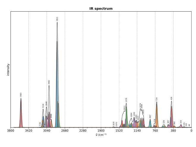
Again we can plot the obtained ir spectra from this simulation, where the same
script we used before can be used again to obtain a spectra:
Wrapping up#
That’s it! You now have access to tools that researchers in computational chemistry use in their day-to-day research :). If you want to learn more, I strongly advise you to first look at the orca input library and the xtb manual in order to see a bit better what these two softwares can do. (spoiler alert: there is a fuckload of things these guys can do) Try not to get overwhelmed, it might feel a like bit like it in the beginning, but it eases up a lot with a little bit of experience.
Next up I plan to write a series of articles showing how we can obtain other spectras like NMR and UV for organic molecules.